Rendering the Mandelbrot Set

Introduction #

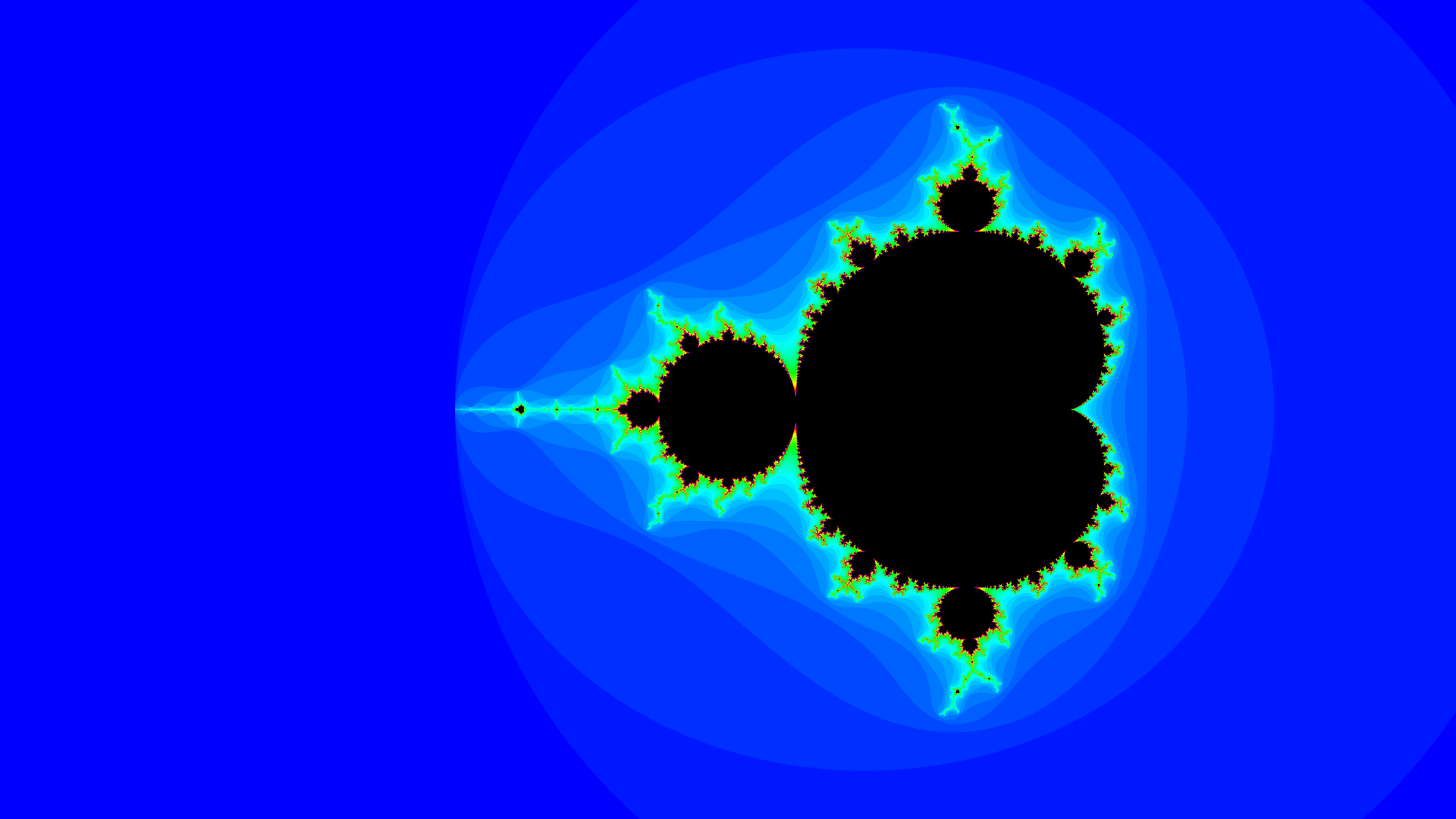
The Mandelbrot set is such a fundamental cool thing™ in doing stuff with computers it seems, and yet I realised I’ve never really tried to actually make one of these cool pictures like up top of this post. I want to rectify that today and answer some questions I had for myself about how to draw it!

Maths basics #

I started by looking at the basic concept. This article over at Mathigon is great. I can’t do better than that for covering the basics. It also gives some hints as to how we can render the Mandelbrot set in the way we are accustomed to seeing it represented.

The fundamental recursive formula that we’re working with is \(z_n = {z_{n-1}}^2 + c\) where \(z_n\) and \(c\) are complex numbers. The Mandelbrot set specifically is the set of values of \(c\) for which the recursive formula does not diverge no matter how many times it is applied, and where \(z_0 = 0\).

The image above represents a 2-dimensional grid where the x axis represents the real part of the complex number \(c\) and the y axis represents the complex part. The colour black is given to values of \(c\) for which the recursive formula does not diverge i.e. the values of \(c\) that are a part of the Mandelbrot set. The colouring of the divergent values of \(c\) is entirely up to us. We’ll see about that later, for now we have enough to get started.

Let’s draw #

I’m going to use Shadertoy to show my code & renders here, because I love it, and it’s very convenient in this case.

Does it diverge? #

First I tried to work out how to determine if the sequence diverges for given \(c\). I got sucked down such a rabbit hole here and spent more than a day digging into the maths. I can’t say I have a solid grasp on it but I’ll try to lay out what I am sure about.

You can play around with this toy that lets you vary \(c\) and trace the values resulting from each iteration of the function as a path to get an intuitive feel for things. There are 3 broad categories of behaviour for different \(c\) you can observe.

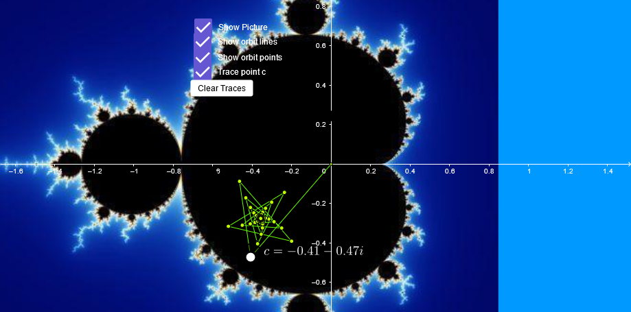
1. \(z_n\) appears to converge on some point in the complex plane.

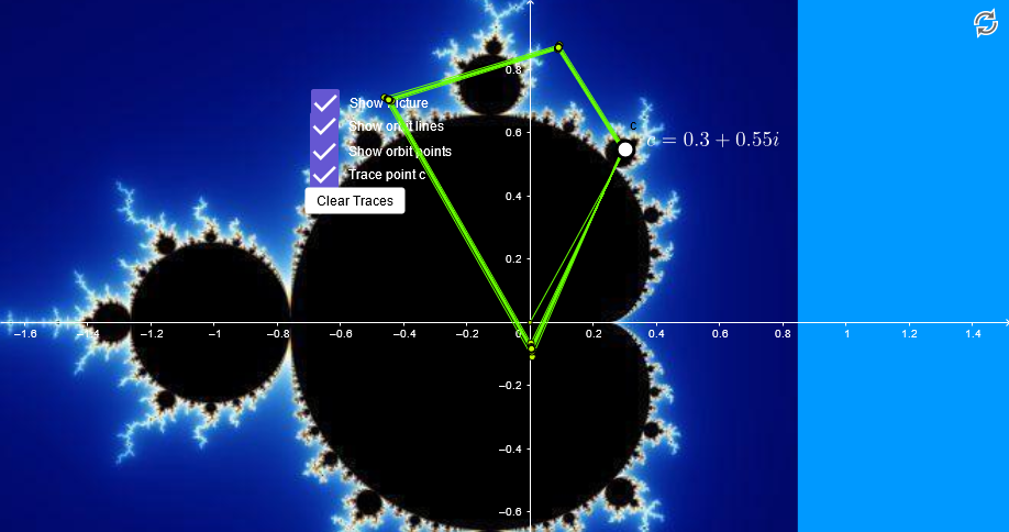
2. \(z_n\) appears to cycle round through some number of points and return to the starting point \(c\).

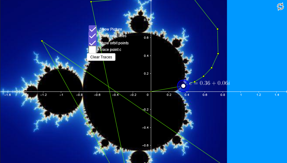
3. \(z_n\) seems to diverge, moving further and further from the origin the more iterations are applied. We expect the magnitude of \(z_\infty\) to be \(\infty\).

We want to know if a particular \(c\) falls into either of the first 2 categories because if it converges on a single point or cycle then it does not diverge.

Sadly the conclusion I took from my time spent digging is: there’s no single easy analytical method for knowing for any possible \(c\) whether it falls into the “converges on a point/cycle” category or into the divergent category. I really wanted an intuitive answer as to why there doesn’t seem to be such a solution given how simple the underlying function is. I didn’t get much satisfaction, but maybe someone can point out why this might be the case. I guess this is a central part of the fascination with the Mandelbrot and Julia sets - that so much complexity arises from such a simple definition. Indeed some sequences particularly close to the boundary of the Mandelbrot set are completely chaotic: tiny changes in the input conditions (\(c\)) cause a large change in the result (whether or not the sequence diverges, and how fast).

It turns out you could study (and people have studied) this behaviour of repeated applications of some function for a lifetime as part of a wider field of Holomorphic Dynamics. I hadn’t really understood this until I saw 3Blue1Brown’s video about this, which I highly recommend if you’re interested:

First stab #

At this point I was little frustrated with having spent so long diving into the maths, I wanted to have something to show for it. So I started by deciding whether a particular \(c\) would diverge by iterating the sequence for some maximum number of steps, and if any element of that sequence ends up outside a certain distance from the origin, assume that it diverges. I’ve chosen an arbitrary large-ish bound.

I colour “divergent” points white and other points black. I’m using scare quotes around “divergent” and being careful not to say “non-divergent points” rather than “other points” because at this point it’s all a bit heuristic and I have no proof about any of it.

Luckily we’ve already got the classic Mandelbrot shape appearing pretty clearly, albeit just a silhouette. There seems to be some interesting artifacting around the main body of the shape (some black spots particulary above and below the x axis), but it could just be aliasing making it appear like artifacts. Either way, it’s a good start.

Here’s the GLSL I ended up with for this first stab:

#define MAX_ITERATIONS 256
#define MAX_DISTANCE 2048.

void mainImage( out vec4 fragColor, in vec2 fragCoord )
{
    // Normalise pixel coordinates (from -limit to +limit)
    float limit = 1.;
    
    float aspect = iResolution.x / iResolution.y;
    vec2 uv = (((fragCoord)/iResolution.xy) * limit * 2.) - limit;
    uv.x *= aspect;
    
    // Offset the x/y coordinates to display because the interesting
    // part of the complex plane in this case is slightly offset to
    // the left.
    vec2 offset_center = vec2(-1.0, 0.0);
    uv += offset_center;
    
    // Setup iteration
    vec2 c = uv;
    // z_1 = c
    vec2 z = uv;
    
    // Does it diverge?
    vec3 col = vec3(0);
    for (int i = 0; i != MAX_ITERATIONS; ++i) {
        // Magnitude of z gives distance from the origin
        float dist = sqrt(dot(z, z));
        if (dist > MAX_DISTANCE) {
            col = vec3(1);
            break;
        }
        
        // f(z) = z^2 + c
        z = vec2(
            z.x * z.x - z.y * z.y,
            2. * z.x * z.y
        ) + c;
    }

    // Output to screen
    fragColor = vec4(col, 1.0);
}

Bounds #

This first stab is pretty unprincipled for several reasons. Firstly I have no evidence that if a point reaches beyond this arbitrary maximum distance that it will actually diverge. Secondly, the specific value I’ve chosen is quite arbitrary, is there a better bound?

I looked at a few resources to understand the following but primarily this question on math.stackexchange and in particular this link.

One condition in which we can be sure the sequence will eventually diverge is to find some conditions under which the distance from the origin \(|z|\) always increases in following iterations. We can write this as follows:

$$ |f(z)| > |z| $$ $$ |z^2 + c| > |z| $$ $$ \frac{|z^2 + c|}{|z|} > 1 $$

We can try to isolate \(|z|\) and \(|c|\) by rearranging this inequality in different ways.

Triangle Inequality for Complex Numbers #

Breaking apart the term \(|z^2 + c|\) into component parts can be done using the triangle inequality.

The easiest way to explain the triangle inequality in this case is to interpret the complex numbers involved as vectors in the complex plane. The sum of 2 complex numbers and the magnitude of a complex number behave the same as vectors in regular 2-dimensional space. This means that placing \(z^2\) starting at the origin, and \(c\) starting from the end of \(z^2\), we can form a triangle out of these 2 vectors and their sum \(z^2 + c\).

Knowing that these 3 vectors can be translated to form a triangle allows us to apply the triangle inequality to \(|z^2|\), \(|c|\) and \(|z^2 + c|\). Using this fact:

$$ \begin{align*} |z^2 + c| + |c| & \ge |z^2| \\ |z^2 + c| & \ge |z^2| - |c| \\ |z^2 + c| & \ge |z|^2 - |c| \text{ (see note below)} \\ \end{align*} $$

If we consider the original inequality we’re trying to satisfy: $$ \begin{align*} \frac{|z^2 + c|}{|z|} & \ge \frac{|z|^2 - |c|}{|z|} & > 1 \\ \frac{|z^2 + c|}{|z|} & \ge |z| - \frac{|c|}{|z|} & > 1\\ \end{align*} $$ We set the middle expression above to be \(> 1\) so that it fits into the original inequality and then continue to try and isolate \(|z|\) and \(|c|\). $$ \begin{align*} |z| - \frac{|c|}{|z|} & > 1 \\ |z| & > 1 + \frac{|c|}{|z|} \\ \end{align*} $$

Here we have some difficulty because we have 2 variables, and one inequality relating them. Much like simulatenous equations, we can’t find a solution for our 2 variables with only a single inequality. We can choose another inequality to use relating the 2 variables, which is equivalent to choosing some subset of the problem where our inequality is satisfied. In this case we choose \(|z| > |c|\) because if \(|z| > |c|\) then \(\frac{|c|}{|z|} < 1\). Plugging this back into our last inequality on \(|z|\) we get: $$ \begin{align*} |z| & > 1 + \frac{|c|}{|z|} \\ |z| & > 1 + 1 \\ |z| & > 2 \\ \end{align*} $$

Putting the above together we have the following inequality:

$$ \begin{align*} |f(z)| > |z| \\ |z^2 + c| > |z| \\ \frac{|z^2 + c|}{|z|} > 1 \\ \end{align*} $$ under the condition that \(|z| > |c|\) and \(|z| > 2\).

So instead of our MAX_DISTANCE cutoff, we have these 2 conditions to satisfy to ensure that a given value of \(c\) will cause the sequence to diverge.

A further bound on \(|c|\) #

We can actually simplify this condition further by checking what happens when \(|c| > 2\), starting from the first iteration in the sequence:

$$ \begin{align*} z_1 & = c \text{ (input to first iteration of sequence)} \\ |f(z_1)| & = |{z_1}^2 + c| = |c^2 + c| \\ |c^2 + c| & \ge |c|^2 - |c| \text{ (by triangle inequality)} \\ |c^2 + c| & \ge |c|(|c| - 1) \\ \end{align*} $$

If we add our condition \(|c| > 2\) then: $$ \begin{align*} |c| - 1 & > 2 - 1 \\ |c| - 1 & > 1 \\ |c|(|c| - 1) & > |c| \\ \end{align*} $$

And lastly putting it all together: $$ \begin{align*} |c^2 + c| \ge |c|(|c| - 1) > |c| \end{align*} $$

This means that so long as \(|c| > 2\) then the following holds: $$ \begin{align*} |f(c)| > |c| \text{ and } |f(c)| > 2 \\ \end{align*} $$ Which matches the conditions we already worked out for when the sequence definitely diverges, so we can say so long as \(|c| > 2\) the sequence diverges.

This finally means we can simplify our condition in code to just check: $$|z_n| > 2$$ For any \(n\) in the sequence because:

• We set \(z_1 = c\) so checking \(|z_n| > 2\) covers the case when \(|c| > 2\) which we’ve just discussed.
• When \(|c| <= 2\) and \(|z_n| > 2\), \(|z_n| > 2 \implies |z_n| > |c|\) so both conditions for divergence are met in this case also.

Let’s draw…better #

Here’s the same thing with #define MAX_DISTANCE 2. Otherwise it’s identical to the first stab, but now I’m happy that the bounds make sense!

Let’s draw…fancier? #

So this is already something, but it’s not the classic vibrant image of the set you might be used to seeing. Now that we understand the process of discovering whether the sequence diverges for each point \(|c|\) in the complex plane \(\mathbb{C}\), we can shade the areas outside of the set in more interesting ways.

For the following I have largely used this wikipedia page as a reference.

Number of steps to diverge #

One thing we can do is shade the areas which diverge in our calculation based on how many iterations they took to diverge. This value is like a rather quantised estimation of the velocity with which the sequence diverges.

This already looks a bit nicer. The core logic for shading the output has now changed to the following:

    // Does it diverge?
    int i = 0;
    for (; i != MAX_ITERATIONS; ++i) {
        // Magnitude of z gives distance from the origin
        float dist = sqrt(dot(z, z));
        if (dist > MAX_DISTANCE) {
            break;
        }
        
        // f(z) = z^2 + c
        z = vec2(
            z.x * z.x - z.y * z.y,
            2. * z.x * z.y
        ) + c;
    }
    
    vec3 col = vec3(0);
    if (i < MAX_ITERATIONS) {
        col = vec3(float(i) / float(MAX_ITERATIONS));
    }

    // Output to screen
    fragColor = vec4(col, 1.0);

So we still shade the areas that do not diverge as black. These areas always reach the maximum number of iterations without hitting our MAX_DISTANCE cutoff. The difference between this and the original shading is the areas that do diverge now have some kind of gradient, even if it’s still not very colourful.

As a bonus, with this method we can visualise how increasing the value of MAX_ITERATIONS causes our rendered silhouette to converge on the true silhouette of the mandelbrot set in quite a satisfying way:

Introduce some colour #

To make things more vibrant, we can map this value to something other than grayscale values. One simple mapping is to take our value i / MAX_ITERATIONS as the hue in a HSV colour value and convert this to RGB. I took the HSV to RGB conversion algorithm from here:

Note that the value of MAX_ITERATIONS we choose has a big impact on the resulting colour profile because every colour is normalised based on this max value, and the points in the plane that will result in a number of iterations close to this max value lie increasingly close to the set boundary. Play around with the value of MAX_ITERATIONS to get a feel for this. Increasing the value will make the above render increasingly dominated by red hues because this is the hue you get when i / MAX_ITERATIONS is zero.

Tweaks and improvements #

At this point I’m happy I’ve got quite a satisfying output image, and a decent understanding of the basics so I’m going to end this exploration here for now. Before stopping I’ve made some other minor improvements/tweaks to the rendering.

Tweaking the colours #

I wanted something less alarming as an image, so the overwhelming red has to go. We can achieve this by offsetting our hue interpretation of the iteration count. Consider that in HSV the hue can be thought of like an angle around a colour wheel:

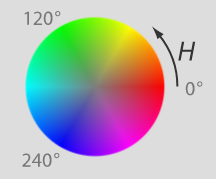
You can see why we end up with a lot of red in our render currently as that is the colour when hue is 0°. We can shift the colour spectrum towards a different colour by shifting this angle. I wanted something bluer like the geogebra toy even if the shading method it uses is probably different so I shifted towards blue which sits at around 240°:

float val = 1. - float(i) / float(MAX_ITERATIONS);
float hue = mod(val * 360.0f + 240.0f, 360.0f);

Note I also took the inverse of i / MAX_ITERATIONS, just because I preferred the colours produced near the boundary of the set (more green rather than fuchsia).

Reducing aliasing #

There is some clear aliasing in the image, particularly where the number of iterations starts increasing more rapidly closer to the set boundary. To mitigate this I did some simple super-sampling by averaging the resulting colour values for more than 1 point around the pixel being shaded. This basically adds a loop around the existing body of the shader, where we calculate the colour at different offsets from the fragment’s cooordinates and take the mean.

The offsets chosen in this case are a regularly spaced grid around the fragment coordinate. I choose a super-sampling rate which applies independently to both x and y dimensions (let’s call it SS_RATE). For example if SS_RATE was 2, we’d take a total of 4 samples for each fragment, 2 in the x axis and 2 in the y axis.

In the regular pixel grid, the distance between fragments is 1 (this is noted in the shadertoy docs). We can determine the distance between samples as the super-sampling rate increases by simply dividing this distance by the rate:

const float sample_distance = 1. / SS_RATE;

We then can determine the offset of each sample from a fragment’s coordinates by considering what a regular grid of points with this spacing would look like overlaid on the original pixel grid. For example if SS_RATE is 2:

Where the larger ‘o’ represents the original fragment coordinates, and ‘·’ represents the super-sampled grid. As a second example when SS_RATE is 3 (please excuse the slightly non-uniform rendering, it’s due to my attempt to plot this out with ascii):

So the offset of the first sample for a fragment is given by calculating the width/height of the sample grid around the fragment coordinate first, and dividing this by 2 to get the offset from the center:

const float sample_distance = 1. / SS_RATE;
const float grid_width = sample_distance * (SS_RATE - 1.);
const float first_sample_offset = -(grid_width / 2.);

Note SS_RATE - 1. in the calculation of grid_width. Consider the width of the square formed by the samples around the fragment in the 2 examples above.

• When SS_RATE is 2 the width of the square is just the distance between 2 samples i.e. 0.5 * 1.
• When SS_RATE is 3 the width of the square is 2 times the distance between 2 samples i.e. 0.333... * 2.

If we extrapolate we see that however many samples we take in each axis the width of that square is sample_distance * (SS_RATE - 1.).

Putting it together in our fragment shader and adding the loop over samples in the square around the fragment we get:

...
#define SS_RATE 4.

void mainImage( out vec4 fragColor, in vec2 fragCoord )
{
    // Super sample and average
    // We have a grid where fragCoord has values from 0.5 to iResolution - 0.5 at intervals of 1 pixel.
    // We pick a super-sampling rate which applies to x and y dimensions independently forming an evenly
    // spaced grid.
    
    const float sample_distance = 1. / SS_RATE;
    const float grid_width = sample_distance * (SS_RATE - 1.);
    const float first_sample_offset = -(grid_width / 2.);
    
    vec3 frag_colour_accum = vec3(0);
    
    for (float sy = 0.; sy < SS_RATE; sy += 1.) {
        for (float sx = 0.; sx < SS_RATE; sx += 1.) {
            
            vec2 sample_coord = vec2(
                fragCoord.x + first_sample_offset + (sample_distance * sx),
                fragCoord.y + first_sample_offset + (sample_distance * sy)
            );

            // ...
            // We do all the original calculations but for
            // sample_coord rather than fragCoord.
            // ...

            
            // Accumulate
            frag_colour_accum += col;
        }
    }
    // The resulting colour is the mean of each of the samples.
    const float total_samples = SS_RATE * SS_RATE;
    fragColor = vec4(frag_colour_accum / total_samples, 1.0);
}

Final render #

Putting together all of the above, this is my final result. I recommend going fullscreen to get a better view:

Summary #

I really enjoyed exploring this topic a bit. This whole topic involves way more maths understanding than I, but a lowly software engineer, had banked on. I spent most of my time trying to work through the maths behind the images, but I think it was worth it!

There’s loads more to explore here, I only really have a very basic result here and there’s lots of improvements I could do. As I said, I’ve run out of steam on this for now. Some improvements I might try at a later date:

• Due to the discrete iteration count being used for shading, we get some obvious stepping between different colour values. We could use a number of different shading methods to smooth this out. There’s some interesting maths here too!
• Other colouring methods - there are a bunch out there, many listed here.
• More advanced rendering methods - for instance Inigo Quilez (one of the creators of shadertoy incidentally) has a nice article describing calculating the distance to the set boundary here as alternative values for shading.

Thanks for reading!